from BPTK_Py import Model
from BPTK_Py import sd_functions as sdCompetitive Pricing Dynamics
Simulation of Competitive Pricing
Competitive Pricing Model
We create our model using the Model class as follows:
model = Model(starttime=0.0,stoptime=2.0,dt=0.25,name='CompetitvePricing')The stock and flow model consists of six parts:
- Production and inventory
- Demand formation
- Price adjustment
- Profit
- Perceived Inventory
- Expected Profitability
The following sections explain each part in more detail. Furthermore, they demonstrate the composition of stocks, flows, converters and constants.
Creating model
1) Production and Inventory

Stocks: production capacity, production, inventory
productionCapacity = model.stock("productionCapacity")
production = model.stock("production")
inventory = model.stock("inventory")
Flows: production start rate, production rate, consumption rate
productionStartRate = model.flow("productionStartRate")
productionRate = model.flow("productionRate")
consumptionRate = model.flow("consumptionRate")
Converters: effect of profitability on capacity utilization,capacity utilization, inventory coverage
capacityUtilization = model.converter("capacityUtilization")
effectOfProfitabilityOnCapacityUtilzation = model.converter("effectOfProfitabilityOnCapacityUtilzation")
inventoryCoverage = model.converter("inventoryCoverage")
Constants: production time
Normalized expected profitability and demand are not constants. They are results of other parts.
productionTime = model.constant("productionTime")2) Demand formation

This model does not have any stocks or flows.
Converters: relative value of product, effect of relative value on demand, reference demand, demand
relativeValueOfProduct = model.converter("relativeValueOfProduct")
effectOfRelativeValueOnDemand = model.converter("effectOfRelativeValueOnDemand")
referenceDemand = model.converter("referenceDemand")
demand = model.converter("demand")
Constants: price of substitutes, size of shock, market shock on
Price is not a constant. It is a result of another part.
sizeOfShock = model.constant("sizeOfShock")
marketShockOn = model.constant("marketShockOn")
priceOfSubstitutes = model.constant("priceOfSubstitutes")
3) Price Adjustment
This section contains two models. The first model determines the minimum price. The second describes the formation of the product’s price.

This model does not have any stocks, flows or constants. Unit variable cost and unit capacity cost are results of other parts.
Converters: capacity cost per unit, minimum price
minimumPrice = model.converter("minimumPrice")
capacityCostPerUnit = model.converter("capacityCostPerUnit")
Stocks: expected price
expectedPrice = model.stock("expectedPrice")Flows: change in expected price
changeInExpectedPrice = model.flow("changeInExpectedPrice")Converters: indicated price, effect of inventory coverage on price, price
indicatedPrice = model.converter("indicatedPrice")
effectOfInventoryCoverageOnPrice = model.converter("effectOfInventoryCoverageOnPrice")
price = model.converter("price")
Constants:
Minimum price and normalized inventory coverage are not constants. Minimum price is a result of the previous model and normalized inventory coverage is a result of another part.
priceAdjustmentTime = model.constant("priceAdjustmentTime")4) Profit

This model has no stocks and flows. Production capacity is not a stock of this part. It is a result of the “Production and Inventory” part from the beginning.
Converters: capacity cost, variable cost, cost, revenue, profit
capacityCost = model.converter("capacityCost")
variableCost = model.converter("variableCost")
cost = model.converter("cost")
revenue = model.converter("revenue")
profit = model.converter("profit")
Constants: unit capacity cost, unit variable cost
Production rate, price and consumption rate are not constants of this model. They are results of other parts. Production rate and consumption rate are converters of the “Production and Inventory” model. Price is a converter of the “Price Adjustment” part.
unitCapacityCost = model.constant("unitCapacityCost")
unitVariableCost = model.constant("unitVariableCost")
5) Perceived Inventory

Stocks: perceived inventory coverage
perceivedInventoryCoverage = model.stock("perceivedInventoryCoverage")Flows: change in perceived inventory coverage
changeInPerceivedInventoryCoverage = model.flow("changeInPerceivedInventoryCoverage")Converters: normalized perceived inventory coverage
normalizedPerceivedInventoryCoverage = model.converter("normalizedPerceivedInventoryCoverage")Constants: inventory coverage perception time, reference inventory coverage
Inventory coverage is not a constant of this part. It is a converter and a result of the “Production and Inventory” model.
referenceInventoryCoverage = model.constant("referenceInventoryCoverage")
inventoryCoveragePerceptionTime = model.constant("inventoryCoveragePerceptionTime")
6) Expected Profitability

Stocks: expected profitability
expectedProfitability = model.stock("expectedProfitability")Flows: change in expected profitability
changeInExpectedProfitability = model.flow("changeInExpectedProfitability")Converters: normalized expected profitability
normalizedExpectedProfitability = model.converter("normalizedExpectedProfitability")Constants: profit adjustment time, reference expected profitability
Profit is not a constant of this part. It is a result of the “Profit” model.
referenceExpectedProfitability = model.constant("referenceExpectedProfitability")
profitAdjustmentTime = model.constant("profitAdjustmentTime")
Initializing the stocks
productionCapacity.initial_value = 200.0
production.initial_value = 300.0
inventory.initial_value = 300.0
expectedPrice.initial_value = 3.0
perceivedInventoryCoverage.initial_value = 3.0
expectedProfitability.initial_value = 100.0
Defining Equations
Production and Inventory
productionTime.equation = 3.0effectOfProfitabilityOnCapacityUtilzation.equation = sd.lookup(normalizedExpectedProfitability,"effectOfProfitabilityOnCapacityUtilzation")
capacityUtilization.equation = effectOfProfitabilityOnCapacityUtilzation
productionStartRate.equation = capacityUtilization*productionCapacity
productionRate.equation = sd.min(production, sd.delay(model, productionStartRate, productionTime, 100.0))
consumptionRate.equation = sd.min(inventory,demand)
inventoryCoverage.equation = inventory/consumptionRateThe stocks production and inventory have inflows and outflows.
production.equation = productionStartRate - productionRate
inventory.equation = productionRate - consumptionRate
We define the effect of profitability on capacity utilzation in our model using a non-linear relationship (depending on the normalized expected profitability). We capture this relationship in a lookup table that we store in the points property of the model (using a Python list):
model.points["effectOfProfitabilityOnCapacityUtilzation"] = [
    [0.0,0.324],
    [0.167,0.33],
    [0.333,0.372],
    [0.5,0.394],
    [0.667,0.41],
    [0.833,0.42],
    [1.0,0.5],
    [1.167,0.745],
    [1.333,0.80075],
    [1.5,0.8565],
    [1.667,0.91225],
    [1.833,0.968],
    [2.0,0.968]
]model.plot_lookup("effectOfProfitabilityOnCapacityUtilzation")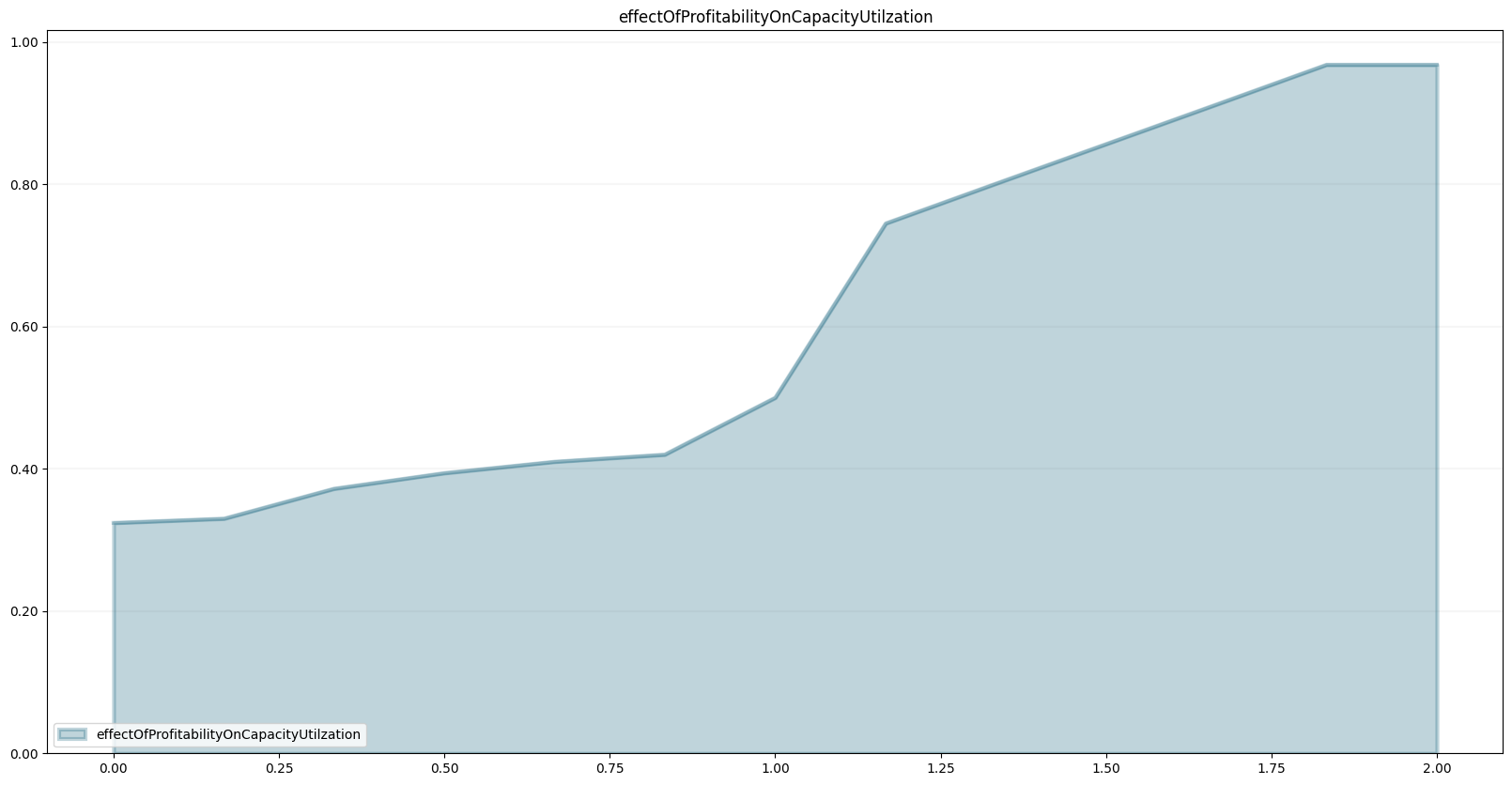
Demand Formation
sizeOfShock.equation = 50.0
marketShockOn.equation = 0.0
priceOfSubstitutes.equation = 3.0
relativeValueOfProduct.equation = priceOfSubstitutes/price
effectOfRelativeValueOnDemand.equation = sd.lookup(relativeValueOfProduct,"effectOfRelativeValueOnDemand")
referenceDemand.equation = 100+marketShockOn*sd.step(sizeOfShock,10.0)
demand.equation = effectOfRelativeValueOnDemand*referenceDemandmodel.points["effectOfRelativeValueOnDemand"] = [
[0.0,0.17],
[0.167,0.191],
[0.333,0.213],
[0.5,0.277],
[0.667,0.351],
[0.833,0.479],
[1.0,1.0],
[1.167,1.362],
[1.333,1.479],
[1.5,1.574],
[1.667,1.638],
[1.833,1.66],
[2.0,1.66]
]model.plot_lookup("effectOfRelativeValueOnDemand")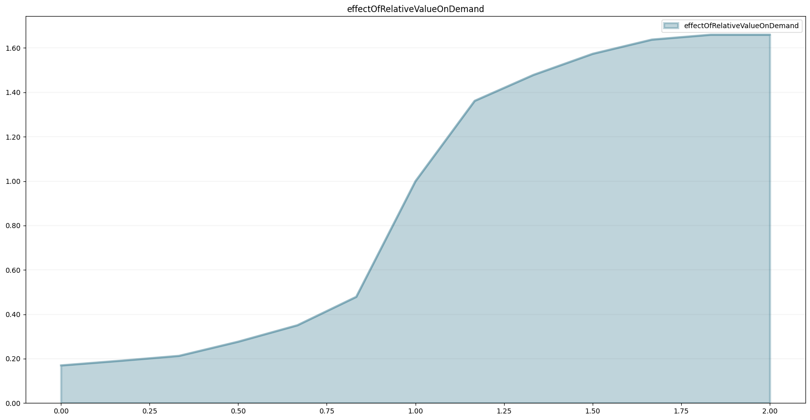
Price Adjustment
priceAdjustmentTime.equation = 3.0capacityCostPerUnit.equation = capacityCost/productionRate
minimumPrice.equation = unitVariableCost+capacityCostPerUnit
effectOfInventoryCoverageOnPrice.equation = sd.lookup(normalizedPerceivedInventoryCoverage,"effectOfInventoryCoverageOnPrice")
price.equation = expectedPrice/effectOfInventoryCoverageOnPrice
indicatedPrice.equation = sd.max(price, minimumPrice)
changeInExpectedPrice.equation = (indicatedPrice-expectedPrice)/priceAdjustmentTimemodel.points["effectOfInventoryCoverageOnPrice"] = [
[0.0,1.404],
[0.167,1.415],
[0.333,1.404],
[0.5,1.372],
[0.667,1.351],
[0.833,1.277],
[1.0,1.0],
[1.167,0.787],
[1.333,0.550],
[1.5,0.4],
[1.667,0.34],
[1.833,0.298],
[2.0,0.298]
]model.plot_lookup("effectOfInventoryCoverageOnPrice")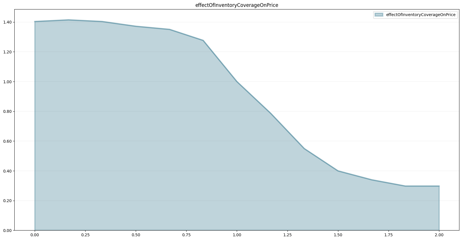
Profit
unitCapacityCost.equation = 0.5
unitVariableCost.equation = 1.0
capacityCost.equation = unitCapacityCost*productionCapacity
variableCost.equation = unitVariableCost*productionRate
cost.equation = variableCost + capacityCost
revenue.equation = price * consumptionRate
profit.equation = revenue - costPerceived Inventory Coverage
referenceInventoryCoverage.equation = 3.0
inventoryCoveragePerceptionTime.equation = 3.0
changeInPerceivedInventoryCoverage.equation = (inventoryCoverage-perceivedInventoryCoverage)/inventoryCoveragePerceptionTime
normalizedPerceivedInventoryCoverage.equation = perceivedInventoryCoverage/referenceInventoryCoverage
perceivedInventoryCoverage.equation = changeInPerceivedInventoryCoverageExpected Profitability
referenceExpectedProfitability.equation = 100.0
profitAdjustmentTime.equation = 12.0
changeInExpectedProfitability.equation = (profit-expectedProfitability)/profitAdjustmentTime
expectedProfitability.equation = changeInExpectedProfitability
normalizedExpectedProfitability.equation = expectedProfitability/referenceExpectedProfitabilityScenario Management
We now use the scenario management of the BPTK-Py framework. We first import the library.
import BPTK_Py
bptk = BPTK_Py.bptk()
Then we set up a scenario manager using a Python dictionary. The scenario manager identifies the baseline constants of the model:
scenario_manager = {
    "smCompetitivePricing":{

    "model": model,
    "base_constants": {
        "marketShockOn":0,
        "sizeOfShock":50

    },
   "base_points":{
            "effectOfProfitabilityOnCapacityUtilization":
            [
                [0.0, 0.324],
                [0.16666666666666666, 0.33],
                [0.3333333333333333, 0.372],
                [0.5, 0.394],
                [0.6666666666666666, 0.41],
                [0.8333333333333334, 0.42],
                [1.0, 0.5],
                [1.1666666666666667, 0.745],
                [1.3333333333333333, 0.80075],
                [1.5, 0.8565],
                [1.6666666666666667, 0.91225],
                [1.8333333333333333, 0.968],
                [2.0, 0.968]
            ],
            "effectOfRelativeValueOnDemand" :
               [
                   [0.0, 0.17],
                   [0.16666666666666666, 0.191],
                   [0.3333333333333333, 0.213],
                   [0.5, 0.277],
                   [0.6666666666666666, 0.351],
                   [0.8333333333333334, 0.479],
                   [1.0, 1.0],
                   [1.1666666666666667, 1.362],
                   [1.3333333333333333, 1.479],
                   [1.5, 1.574],
                   [1.6666666666666667, 1.638],
                   [1.8333333333333333, 1.66],
                   [2.0, 1.66]
               ]
            ,
             "effectOfInventoryCoverageOnPrice" :
                  [
                      [0.0, 1.404],
                      [0.16666666666666666, 1.415],
                      [0.3333333333333333, 1.404],
                      [0.5, 1.372],
                      [0.6666666666666666, 1.351],
                      [0.8333333333333334, 1.277],
                      [1.0, 1.0],
                      [1.1666666666666667, 0.787],
                      [1.3333333333333333, 0.55],
                      [1.5, 0.4],
                      [1.6666666666666667, 0.34],
                      [1.8333333333333333, 0.298],
                      [2.0, 0.298]
                  ]
        },
        "scenarios":{
             "base":{
              }
        }

 }
}
The next step is to register the scenario manager as follows:
bptk.register_scenario_manager(scenario_manager)Once we have this, we can define and register more scenarios as follows:
bptk.register_scenarios(
    scenarios =
        {
             "marketShock":{
                "constants":{
                    "marketShockOn":1
                }
            },
              "availabilityLoop":{
               "constants":{
                    "marketShockOn":1
                },
               "points":{
                      "effectOfProfitabilityOnCapacityUtilization" :
                       [
                           [0.0, 0.5],
                           [0.16666666666666666, 0.5],
                           [0.3333333333333333, 0.5],
                           [0.5, 0.5],
                           [0.6666666666666666, 0.5],
                           [0.8333333333333334, 0.5],
                           [1.0, 0.5],
                           [1.1666666666666667, 0.5],
                           [1.3333333333333333, 0.5],
                           [1.5, 0.5],
                           [1.6666666666666667, 0.5],
                           [1.8333333333333333, 0.5],
                           [2.0, 0.5]
                       ],
                    "effectOfRelativeValueOnDemand" :
                    [
                        [0.0, 1.0],
                        [0.16666666666666666,1.0],
                        [0.3333333333333333, 1.0],
                        [0.5, 1.0],
                        [0.6666666666666666, 1.0],
                        [0.8333333333333334, 1.0],
                        [1.0, 1.0],
                        [1.1666666666666667, 1.0],
                        [1.3333333333333333,1.0],
                        [1.5, 1.0],
                        [1.6666666666666667,1.0],
                        [1.8333333333333333, 1.0],
                        [2.0, 1.0]
                    ],
                     "effectOfInventoryCoverageOnPrice" :
                        [
                            [0.0, 1.0],
                            [0.16666666666666666, 1.0],
                            [0.3333333333333333, 1.0],
                            [0.5, 1.0],
                            [0.6666666666666666, 1.0],
                            [0.8333333333333334, 1.0],
                            [1.0, 1.0],
                            [1.1666666666666667, 1.0],
                            [1.3333333333333333, 1.0],
                            [1.5, 1.0],
                            [1.6666666666666667, 1.0],
                            [1.8333333333333333, 1.0],
                            [2.0, 1.0]
                        ]
               }

           },
           "capacityUtilizationLoop":{
               "constants":{
                    "marketShockOn":1
                },
               "points":{

                    "effectOfRelativeValueOnDemand" :
                    [
                        [0.0, 1.0],
                        [0.16666666666666666,1.0],
                        [0.3333333333333333, 1.0],
                        [0.5, 1.0],
                        [0.6666666666666666, 1.0],
                        [0.8333333333333334, 1.0],
                        [1.0, 1.0],
                        [1.1666666666666667, 1.0],
                        [1.3333333333333333,1.0],
                        [1.5, 1.0],
                        [1.6666666666666667,1.0],
                        [1.8333333333333333, 1.0],
                        [2.0, 1.0]
                    ]

           }
           },
             "substitutionLoop":{
               "constants":{
                    "marketShockOn":1
                },
               "points":{
                      "effectOfProfitabilityOnCapacityUtilization" :
                       [
                           [0.0, 0.5],
                           [0.16666666666666666, 0.5],
                           [0.3333333333333333, 0.5],
                           [0.5, 0.5],
                           [0.6666666666666666, 0.5],
                           [0.8333333333333334, 0.5],
                           [1.0, 0.5],
                           [1.1666666666666667, 0.5],
                           [1.3333333333333333, 0.5],
                           [1.5, 0.5],
                           [1.6666666666666667, 0.5],
                           [1.8333333333333333, 0.5],
                           [2.0, 0.5]
                       ]
               }

           }
        }
    ,
    scenario_manager="smCompetitivePricing")
Using the plot_lookup function on the bptk class, we can compare the lookup functions between different scenarios.
bptk.plot_lookup(
    scenario_managers=["smCompetitivePricing"],
    lookup_names=["effectOfProfitabilityOnCapacityUtilization"],
    scenarios=["base","availabilityLoop"])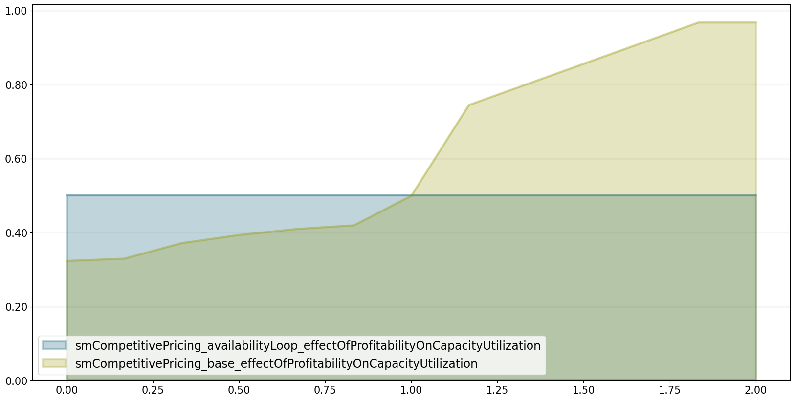
Scenario Experiments
Base Case
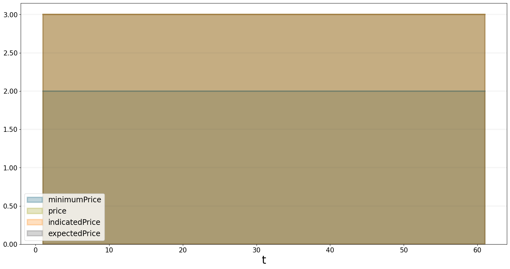
Let’s quickly run through the base case first, which starts the model in equilibrium.
The equilibrium price for our product is set at EUR 3. This is equal to both the indicated price and the expected price. The minimum price (the amount we need to be profitable) is at EUR 1.5
bptk.plot_scenarios(
            scenario_managers=["smCompetitivePricing"],
            scenarios=["base"],
            equations=["minimumPrice","price","indicatedPrice","expectedPrice"]
            )
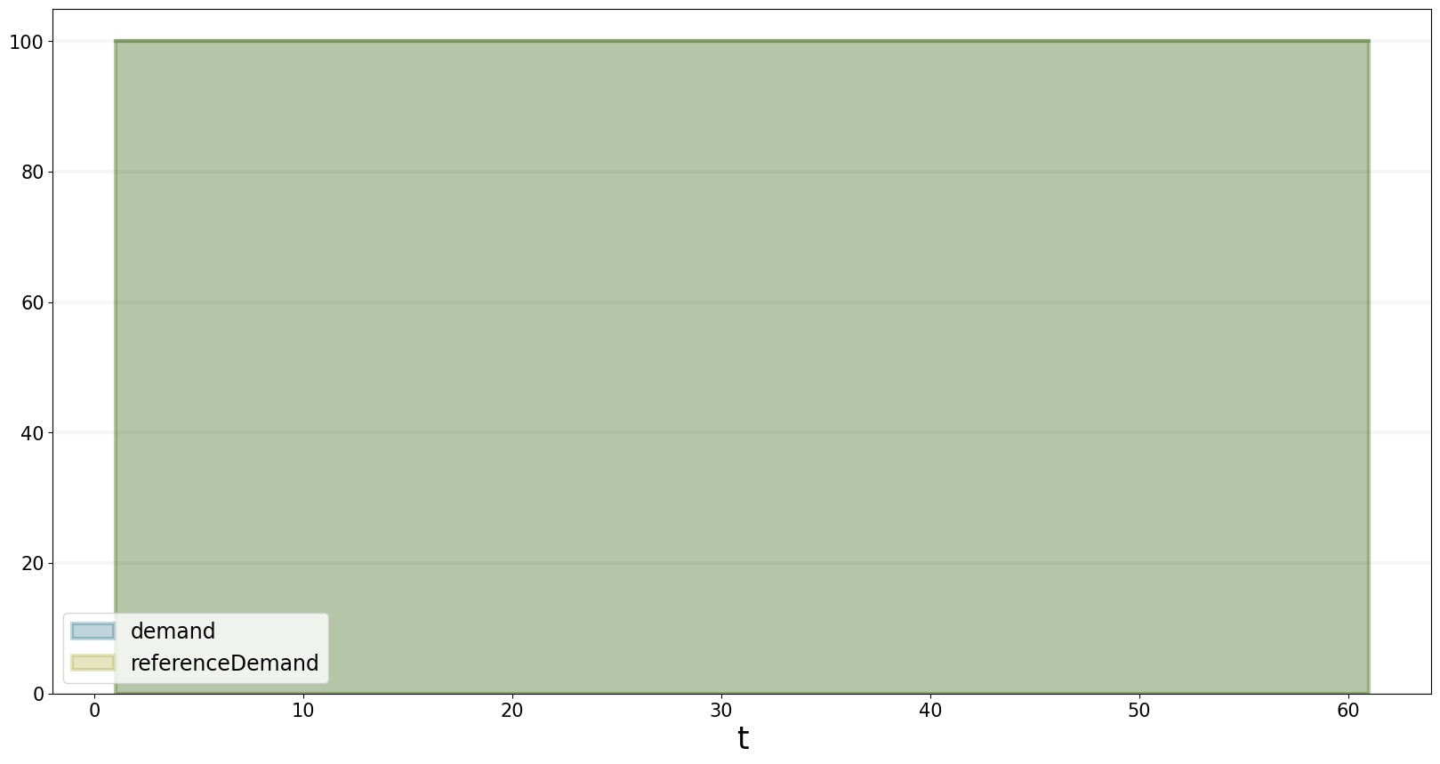
Initially there is a reference demand of 100 units per month. Because the market is in equilibrium, the reference demand (i.e. the demand given the equilibrium price) equals the actual demand.
bptk.plot_scenarios(
            scenario_managers=["smCompetitivePricing"],
            scenarios=["base"],
            equations=["demand","referenceDemand"]
            )
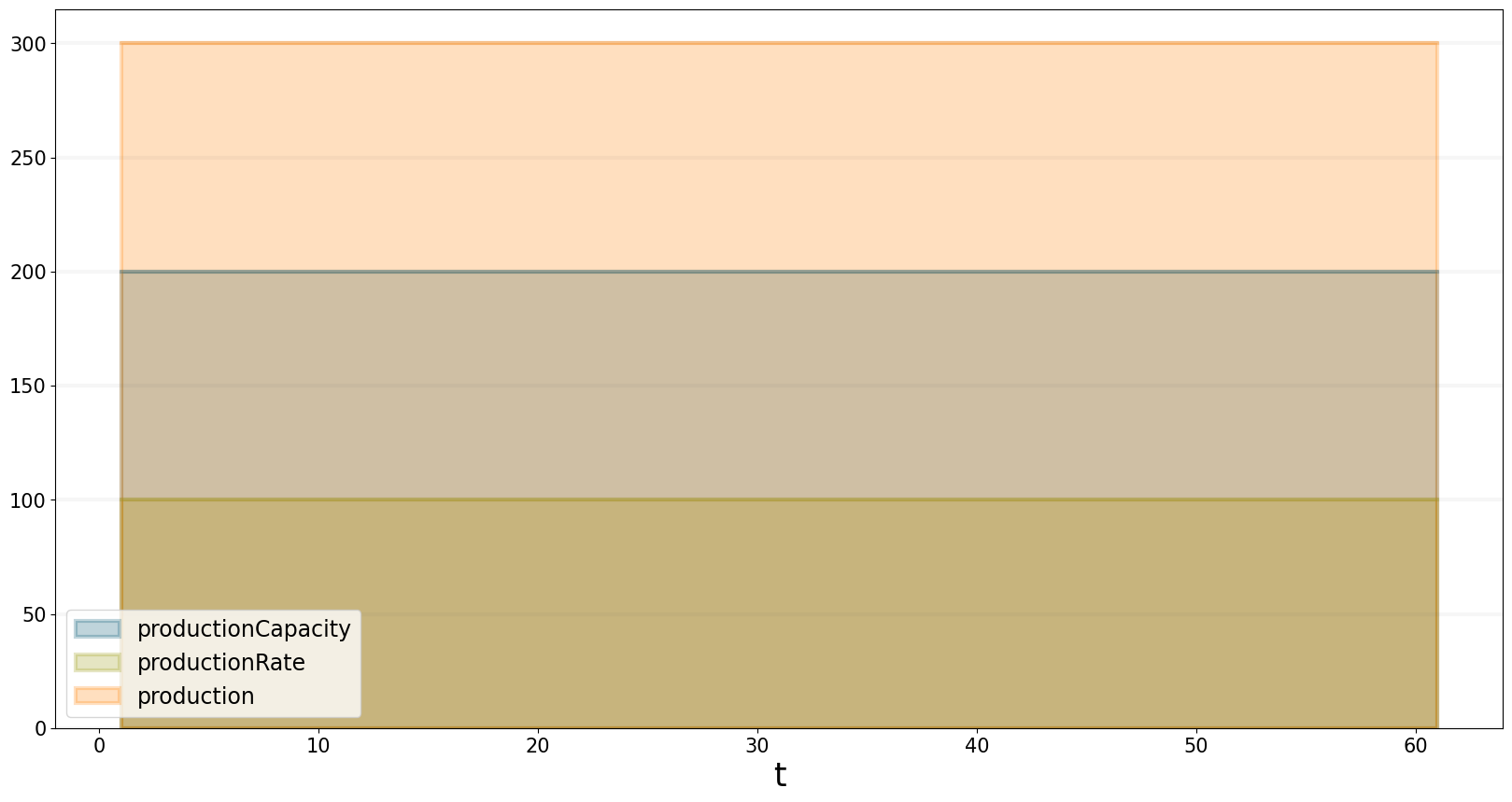
Our production capacity is 200 units per month - but we only produce 100 units per month to avoid overstocking and are thus at a utilization of 50%. 300 units are “work in progress” within production.
bptk.plot_scenarios(
            scenario_managers=["smCompetitivePricing"],
            scenarios=["base"],
            equations=["productionCapacity","productionRate","production"]
            )
Capacity utilization is thus at 50%.
bptk.plot_scenarios(
            scenario_managers=["smCompetitivePricing"],
            scenarios=["base"],
            equations=["capacityUtilization"]
            )
The inventory is also at 300 and the consumption rate equals the demand, i.e. is at 100.
bptk.plot_scenarios(
            scenario_managers=["smCompetitivePricing"],
            scenarios=["base"],
            equations=["inventory","consumptionRate"]
            )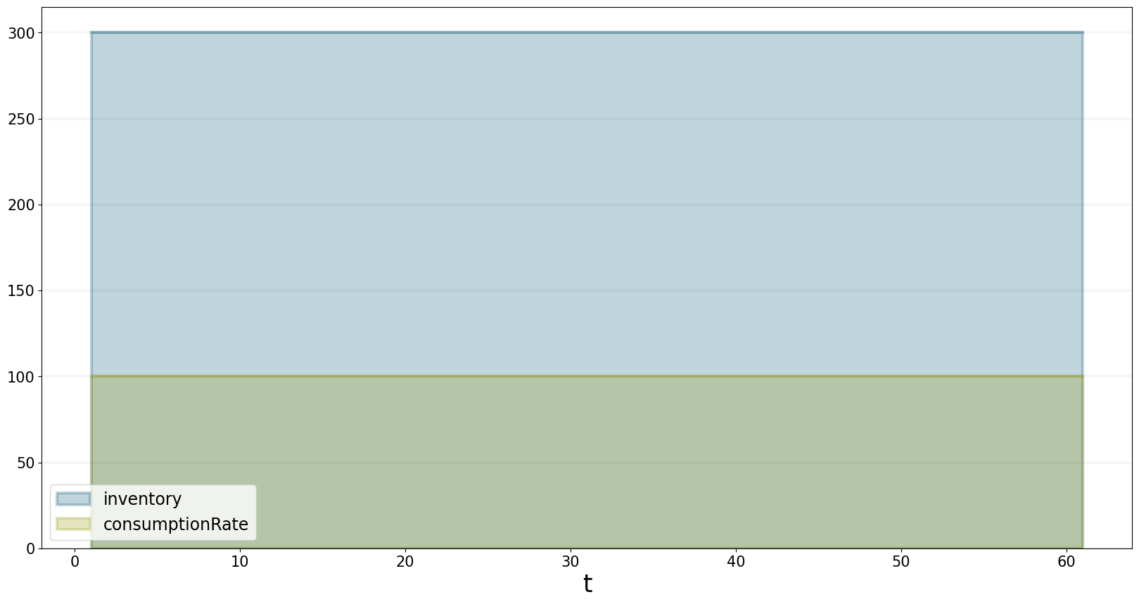
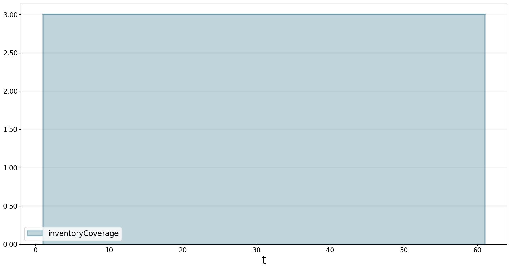
This leads to an inventory coverage of 3.
bptk.plot_scenarios(
            scenario_managers=["smCompetitivePricing"],
            scenarios=["base"],
            equations=["inventoryCoverage"]
            )
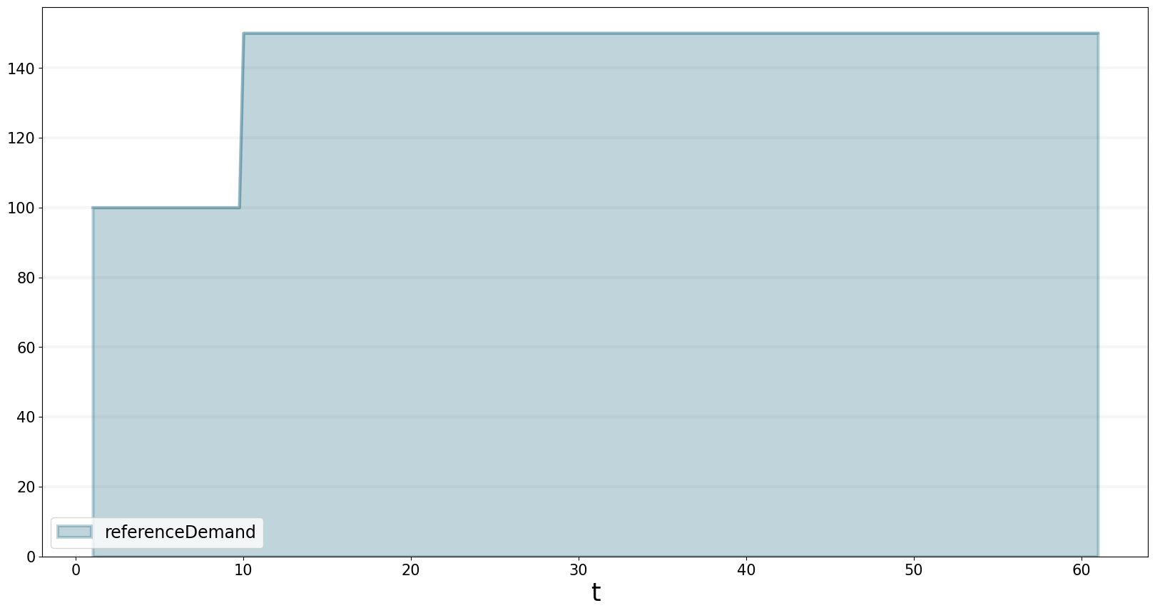
Market Shock
Let’s investigate what happens if there is a sudden increase in the underlying demand of 50% at timestep 10. Note that the increase in demand is at the current level of pricing.
bptk.plot_scenarios(
            scenario_managers=["smCompetitivePricing"],
            scenarios=["marketShock"],
            equations=["referenceDemand"]
            )
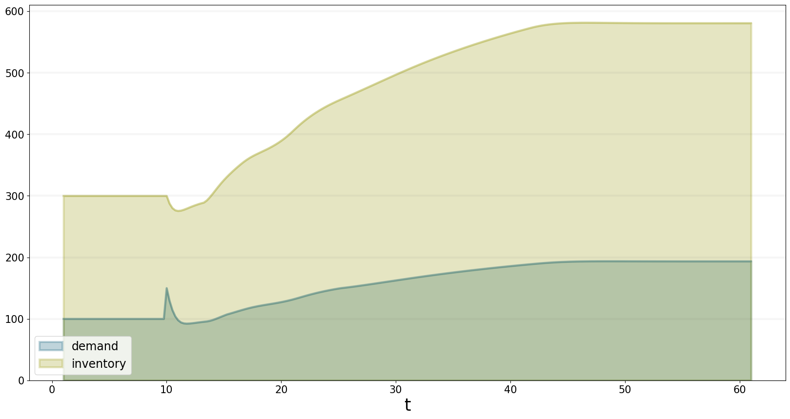
The graph below shows how the actual demand and the inventory develops - as expected, there is an inital demand peak. But this causes the inventory to drop, which increases the price. The increase price leads to increased production, which then lowers the price and thus increases demand.
bptk.plot_scenarios(
            scenario_managers=["smCompetitivePricing"],
            scenarios=["marketShock"],
            equations=["demand", "inventory"]
            )
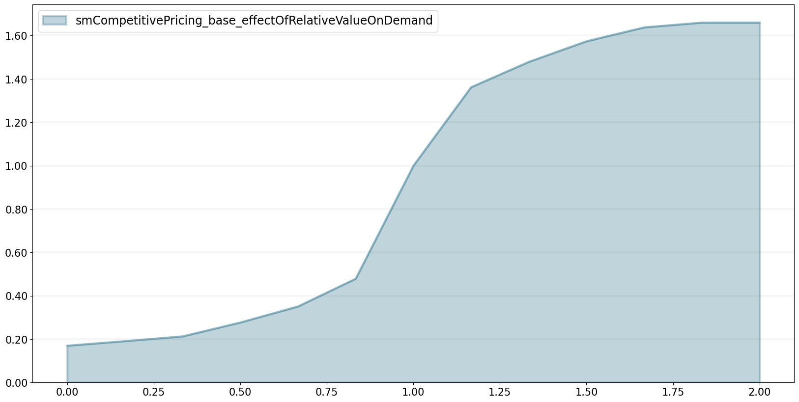
This is because the actual price affects the demand - if the price is higher then the reference price, demand drops, if the price is lower, demand increases compared to the reference demand.
The plot below shows how the dependency is quantified in this model using a non-linear function - the exact shape of this function will depend on your specific situation.
bptk.plot_lookup(
            scenario_managers=["smCompetitivePricing"],
            scenarios=["base"],
            lookup_names=["effectOfRelativeValueOnDemand"]
)
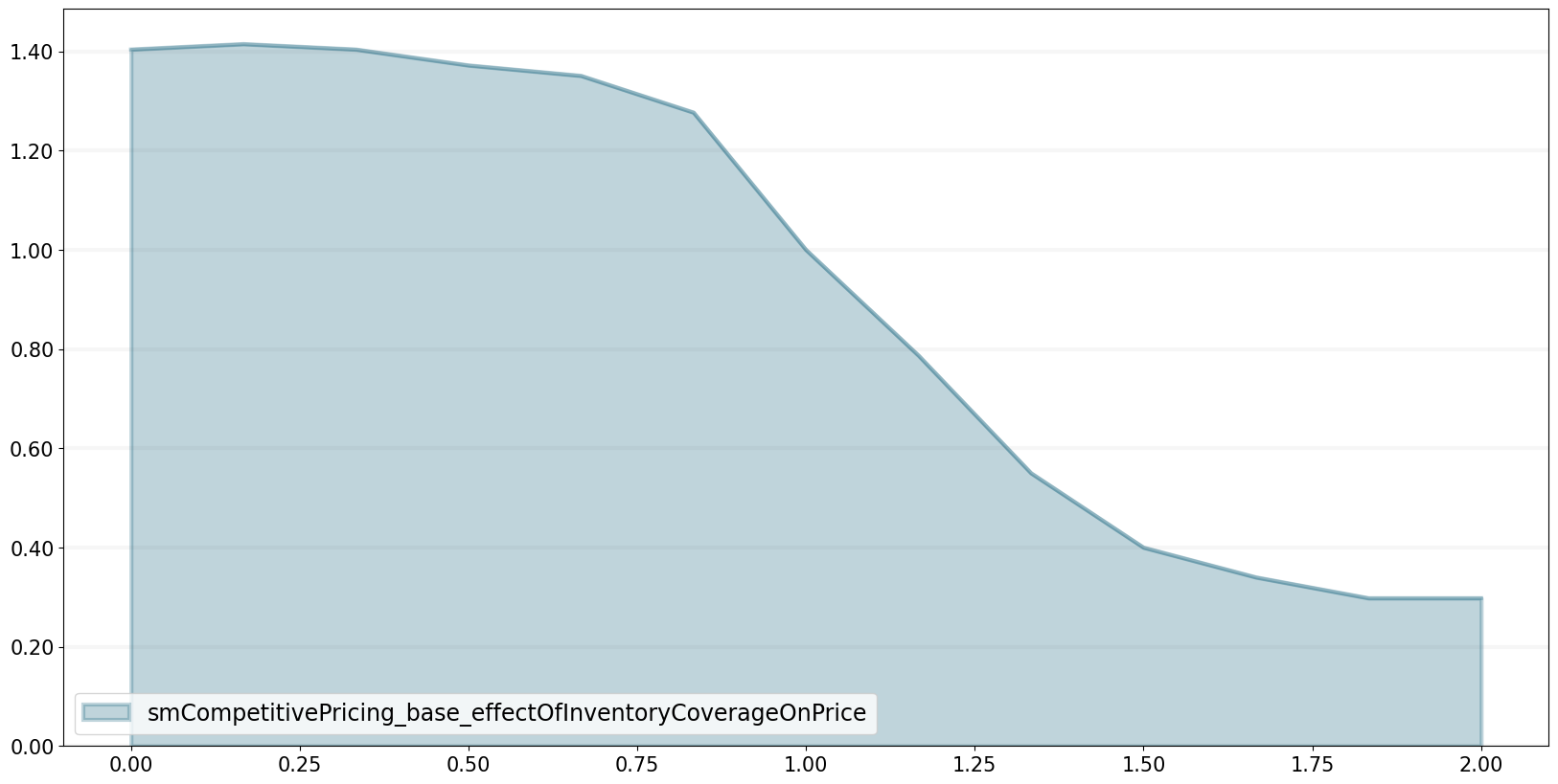
We also assume that prices are sensitive to the availability of the product. If the product becomes scare (i.e. the inventory coverage falls), prices go up, and vice versa. The dependency is modelled using the following table function:
bptk.plot_lookup(
            scenario_managers=["smCompetitivePricing"],
            scenarios=["base"],
            lookup_names=["effectOfInventoryCoverageOnPrice"]
)
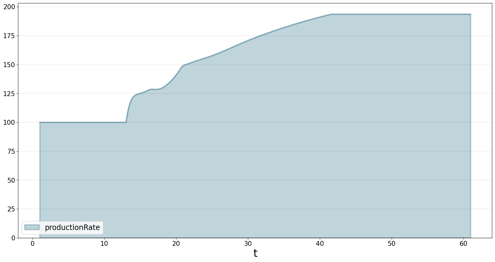
The production rate increases to a new, much higher level.
bptk.plot_scenarios(
            scenario_managers=["smCompetitivePricing"],
            scenarios=["marketShock"],
            equations=['productionRate']
            )
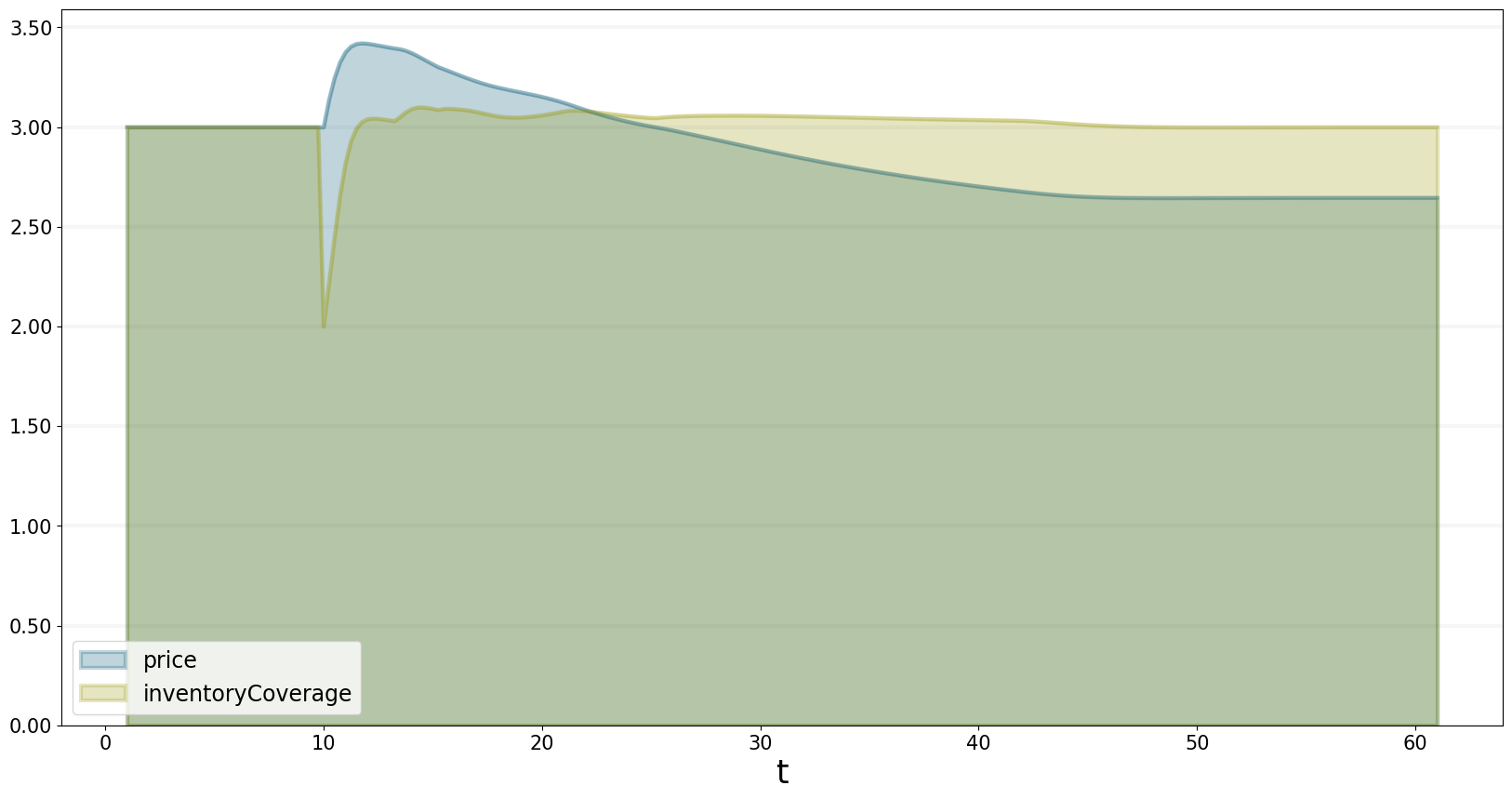
The price increases initially, because of the drop in inventory coverage. But the inventory coverage quickly recoveres due to increase production. Because inventory coverage influences the price, this leads to a price that is actually lower than the original price, but also to a demand that is higher than that indicated by the initial market shock.
bptk.plot_scenarios(
            scenario_managers=["smCompetitivePricing"],
            scenarios=["marketShock"],
            equations=['price','inventoryCoverage']
            )
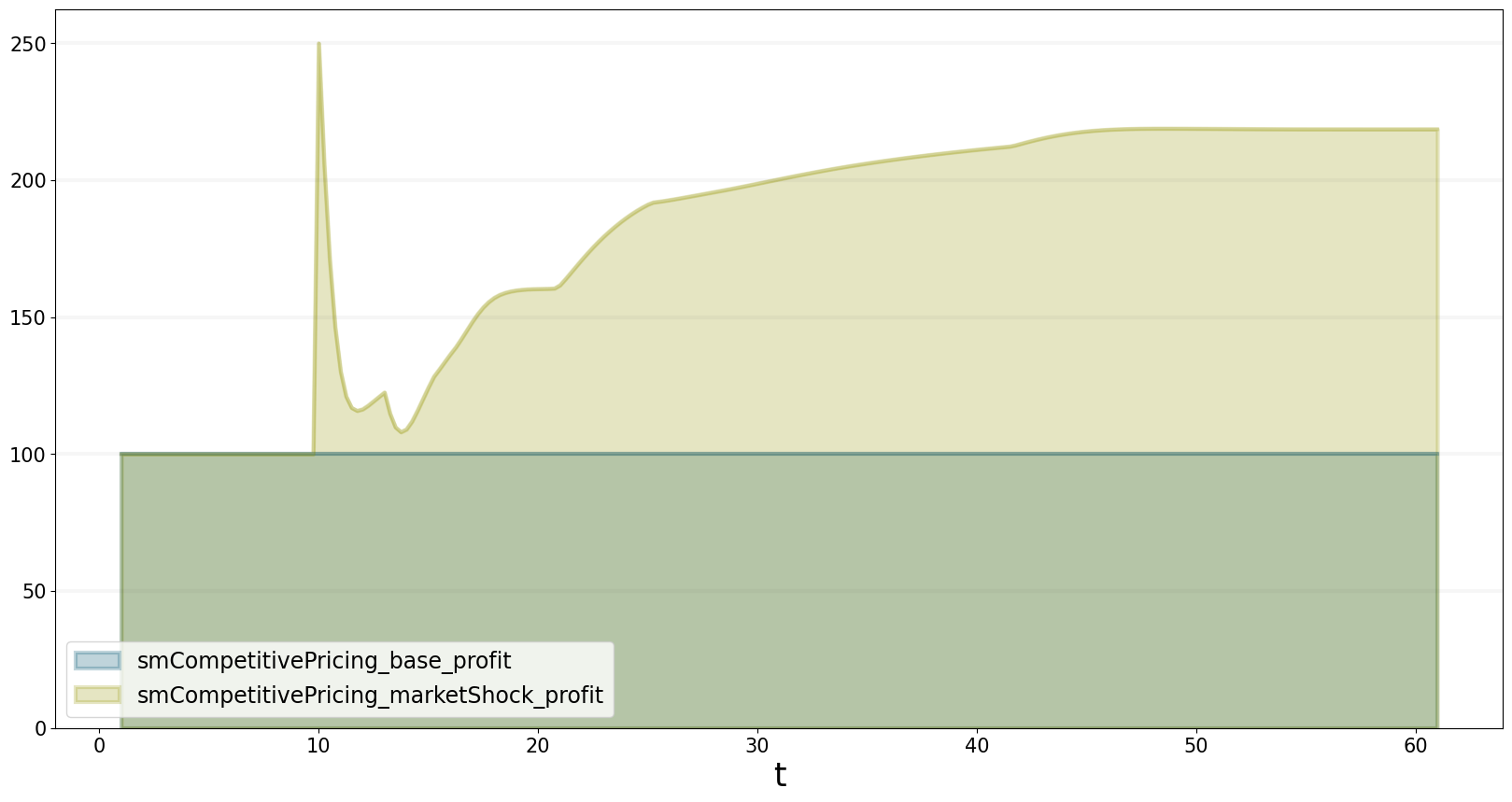
even though the overall demand incrase is only at around 75%, our profits more than double, as seen in the graph below.
bptk.plot_scenarios(
            scenario_managers=["smCompetitivePricing"],
            scenarios=["base","marketShock"],
            equations=['profit']
            )
This is because we are utilizing our production capacity better: we go from a utilization of 50% to a utilization above 90%, as seen in the graph below.
bptk.plot_scenarios(
            scenario_managers=["smCompetitivePricing"],
            scenarios=["base","marketShock"],
            equations=['capacityUtilization']
            )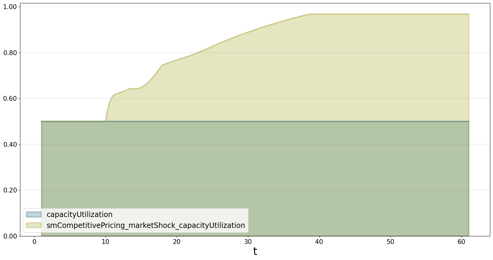
The figures above show that with the given shock of a 50% increase in underlying demand, we get close to our capacity limits.