Using the XMILE Compiler Standalone

In-depth explanation of how to use the XMILE Compiler Standalone.

Using the XMILE Compiler Standalone

The BPTK-Py package contains a compiler which compiles System Dynamics models that use the XMILE format into Python code. This means that you can compile models created with Stella, iThink or Vensim (via the XMILE export) into Python code which will then run standalone.

The result of the compilation is a Python class that only depends on NumPy and SciPy. This class contains the entire simulation model and it can run “standalone”, i.e you don’t need the BPTK framework to actually run the simulation and extract simulation results.

Running models standalone can be useful if want to run your model many times with different initial setting, e.g. for machine learning experiments. In such cases you don't need the extra functionality provided by the frameworks bptk class and it is more efficent to work with the raw simulation model.

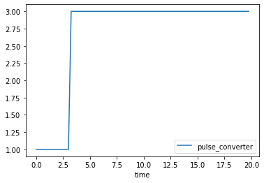
To illustrate this, let's assume we have a small XMILE model called test_compiler.stmx that lives in the simulation_models folder. The model contains one converter called pulse_converter with the following equation:

1+PULSE(0.5, 3.25)

Then all we need to convert the file into a python file test_compiler.py is the following:

from BPTK_Py.sdcompiler.compile import compile_xmile
src = "./simulation_models/test_compiler.stmx"
dest = "./simulation_models/test_compiler.py"
target = "py"

compile_xmile(src, dest, target)

The generated file contains everything you need to run the model, the model itself is in a class simulation_model. That class contains a number of generic methods that are needed for system dynamics simulations, such as simulation_model.delay or simulation_model.random_with_seed. These methods are always generated, irrespective of whether your model actually uses them. This ensures that all generated simulation_model classes have the same methods.

Your models equations themselves are stored in the class as a dictonary of lambda functions. As our example model only contains one converter called pulse_converter, our equations dictionary will also only contain one such converter:

from simulation_models.test_compiler import simulation_model

model = simulation_model()

model.equations

{'pulseConverter': <function simulation_models.test_compiler.simulation_model.__init__.<locals>.<lambda>(t)>}

Because equations are Python Lambda functions that take time t as an argument, we can call these functions directly:

model.equations["pulseConverter"](5.25)

3.0

The simulation_model doesn’t have any “convenience” functions to plot the equations (because those functions are provided by the frameworks bptk class).

But you can easily generate data into a pandas dataframe and then plot that data using the dataframe’s plot() method:

from numpy import arange
data=[[x,model.equations["pulseConverter"](x)] for x in arange(0,20,0.25)] 

import pandas as pd
df = pd.DataFrame(data,columns=["time","pulse_converter"])
df=df.set_index("time")
df[2:5] # just showing an interesting subset of data here

	pulse_converter
time
2.00	1.0
2.25	1.0
2.50	1.0
2.75	1.0
3.00	1.0
3.25	3.0
3.50	3.0
3.75	3.0
4.00	3.0
4.25	3.0
4.50	3.0
4.75	3.0
5.00	3.0

df.plot()

image