Deterministic Functions
system dynamics, systemdynamics, sd dsl, bptk, bptk-py, python, business simulation
Deterministic Functions
The functions of the SD DSL that give the same result on every run, from A to Z. To use them, import sd_functions beside the Model class:
ABS Function
The ABSfunction returns the absolute value of its input.
Signature: abs(input)
input may be any model element.
CEIL / FLOOR / TRUNC Functions
ceil rounds its input up to the next whole number, floor rounds it down. Unlike round they take no digit count - they always go to the nearest integer, and they always go in the same direction.
Signature: ceil(expression), floor(expression) and trunc(expression)
expression can be any element that returns a float value.
trunc(expression) cuts off the fractional part instead, towards zero. For a negative number that is the other direction: floor(-2.5) is -3, trunc(-2.5) is -2. The XMILE builtin INT is floor.
The example divides time by three, so the two functions step at different moments:
CGROWTH Function
CGROWTH turns a growth rate per time unit, in percent, into the rate per dt that compounds to it. A stock whose inflow is stock * cgrowth(model, 10) grows by 10 percent per time unit, whatever dt is - with stock * 0.10 it grows faster the smaller dt is. The example runs both with dt = 0.25: after ten time units compounded stands at 259, which is 100 × 1.1¹⁰, and simple above it.
Signature: cgrowth(model, percentage)
COMBINATIONS
The COMBINATIONS operator calculates the number of r-element subsets (or r-combinations) of an n-element set without repetition.
Arguments n and r must follow n >= r >= 0 and be integers.
Example using n as time - because n must be an integer, we have to wrap it in a user defined function.
COUNTER Function
COUNTER describes a cycle in time: it starts at start at STARTTIME, rises by one per time unit and falls back to start on reaching end.
Signature: counter(model, start, end)
DELAY Function
The DELAY function returns a delayed value of input, using a fixed lag time of delay duration, and an optional initial value initial for the delay. If you don’t specify an initial value initial, DELAY assumes the value to be the initial value of input. A delay duration that changes during the run is read at every step, so the lag follows it - Stella fixes it at its initial value instead
Signature: delay(model, input_function, delay_duration, initial_value)
Each argument can be a number, a model element or an expression.
DELAY1 / DELAY3 / DELAYN Functions
DELAY1, DELAY3 and DELAYN are material delays of first, third and n-th order: what goes in comes out again, spread over time. delay1 is one stock that drains at its content divided by the delay time. delay3 and delayn chain three or n such stocks, each with its share of the delay time, so the output starts later and rises more steeply - the higher the order, the closer it comes to DELAY.
With a constant delay time they behave exactly like SMOOTH, SMOOTH3 and SMOOTHN. When the delay time changes they do not: a material delay passes on everything that went in, a smooth does not.
Signatures: delay1(model, input_function, delay_time, initial_value=None), delay3(model, input_function, delay_time, initial_value=None) and delayn(model, input_function, delay_time, order, initial_value=None)
delay_time: any model element
initial_value: the output at the start, a number, a model element or an expression. Left out, the delay starts at the input
order: a whole number between 1 and 255. delayn keeps every stage at least one dt long, so a delay shorter than order * dt is lengthened to that, as in Stella
DERIVN Function
DERIVN is the n-th derivative of a variable over time, taken as repeated differences over one dt. It is 0 for the first order steps, because there is no earlier value to take a difference from.
Signature: derivn(model, variable, order)
order: a whole number of at least 0
DT Function
The DT function returns the models dt..
Signature: dt(model)
EXP Function
The exp function returns the exponential value of the input.
Signature: exp(element)
element can be any model element (stock, flow, converter, constant)
FACTORIAL Function
The FACTORIAL function calculates the factorial of the single argument n (traditionally noted as n!). n must be an integer value, decimal values are not allowed.
The following example wraps the time t in a user-defined function to ensure that this value is always an integer.
FORECAST Function
FORECAST extrapolates the input over a horizon with its trend: input * (1 + trend * horizon), where the trend is that of TREND with the same averaging time and initial trend.
Signature: forecast(model, input_function, averaging_time, horizon, initial_trend=0.0)
averaging_time, horizon: any model element
initial_trend: the trend at the start, a number, a model element or an expression
GAMMALN Function
The GAMMALN operator returns the natural log of the GAMMA function, given input n. The GAMMA function is a continuous version of the FACTORIAL builtin, with GAMMA(n) the same as FACTORIAL(n-1).
Only argument is n
IF / THEN / ELSE / AND / NOT / OR
It is possible to write up if clauses. We even support NOT and AND / OR operators.
Please note that these function names begin with a capital letter. This is because the actual words if, and, or etc. are protected in Python and cannot / should not be overwritten.
An if clause requires 3 arguments: If ( <condition> , <then>, <else>)
condition: Must be a boolean expression, e.g. sd.time() > 1 is true iff the simulation time is larger than 1 then : Any expression that returns a float value if the condition is true else : Any expression that returns a float value if the condition is false
A simple if clause may look like this:
You see that its value is 5 until t reaches 6.
You can also add and / or / not conditions easily:
Signature: And(<condition1>, <condition2>) : Logical and between 2 conditions Or(<condition1>, <condition2>) : Logical or between 2 conditions Not(<condition>) : Logical not: True if condition is False
Each condition within the operators has to return a boolean value. Nesting of the operators is easily possible!
INIT / PREVIOUS / HISTORY Functions
Three ways to read what a variable was earlier in the run. init is its value at the start. previous is its value one dt back, and initial_value at the first step - which also lets a variable refer to its own last value, as XMILE’s PREVIOUS(SELF, ...) does. history is its value at a given time; for a time after the current one or before the start it gives 0, as Stella does.
Signatures: init(model, variable), previous(model, variable, initial_value) and history(model, variable, time)
variable is a model element or an expression; initial_value and time can be numbers, model elements or expressions.
INVNORM Function
The INVNORM operator calculates the inverse of the NORMALCDF function (see below): the value below which a share p of a normal distribution lies.
Parameters are the probability p (between 0 and 1), and optionally the mean (default 0) and the stddev (default 1). Either of the two may be given without the other.
Example:
IRR Function
IRR is the internal rate of return of a stream of payments so far: the rate at which their net present value is zero, each value discounted by (1 + rate) ** (TIME - STARTTIME). The stream needs payments in both directions. Where there are several such rates the one nearest zero is taken, and where there is none - at the first step, or for a stream that only ever pays in - the function gives missing, or NaN without one. It does not run on the Rust engine yet.
The example pays 100 in the first year and gets 10 back every year after. The rate of return starts deep below zero and climbs towards 10 percent as the payments go on.
Signature: irr(model, stream, missing=None)
LN / LOG10 Functions
ln returns the natural logarithm of its input, log10 the logarithm to base 10.
Signature: ln(expression) and log10(expression)
expression can be any element that returns a positive float value - the logarithm of zero or of a negative number is undefined, so make sure your input stays above zero over the whole simulation period.
The example below starts at t = 1 for exactly that reason:
LOOKUP Function
lookup evaluates a graphical function: a relationship you give as a list of points rather than as a formula. Between two points the value is interpolated linearly; outside the given range it stays at the first or last point.
Signature: lookup(element, points)
element is the input to look up, points a list of (x, y) tuples, in any order - they are sorted by x. Two points at the same x are refused with an error naming it, since the table would have two values there.
This is the DSL equivalent of a graphical function in a XMILE model, and it is the right tool whenever a relationship is known empirically but has no closed form:
LOOKUPINV / LOOKUPAREA Functions
lookupinv reads a lookup table backwards: the x at which it reaches a value. It is meant for a table that only rises or only falls; a value beyond what the table reaches gives the x of the nearer end. lookuparea is the area under the table between two x values, or under all of it.
Signatures: lookupinv(value, points) and lookuparea(points, from_x=None, to_x=None)
points is a list of (x, y) points or the name of a table in model.points, as for lookup. Neither function runs on the Rust engine yet.
The example feeds the time into the same table three ways: forwards reads it as lookup does, backwards asks at which x the table reaches the time, and area_so_far is the area under the table from 0 to the time. Past the last point at x = 4 the table stays at 6, so backwards stops at 4 once the time reaches 6, and the area grows by 6 per time unit.
MAX Function
The max function always chooses the largest of its input values - two or more.
Signature: max(element, element, ...)
element can be any model element (stock, flow, converter, constant)
MIN Function
The min function always chooses the smallest of its input values - two or more.
Signature: min(element, element, ...)
element can be any model element (stock, flow, converter, constant)
NAN / INF / PI
sd.nan() returns a NAN value, sd.Inf() gives you the infinity value, sd.pi() returns the number pi.
NORMALCDF Function
The NORMALCDF operator calculates the cumulative Normal distribution function between the specified z-scores, or, when the mean and stddev (standard deviation) are given, between two data values.
Arguments are the left and right boundaries and optionally mean and stddev. If not given, mean will be set to 0, stddev to 1.
A really simple example:
NPV Function
NPV accumulates the net present value of a stream: in every step the input, discounted by 1 / (1 + rate) ** (TIME - STARTTIME + DT), is added. rate is the discount rate per time unit of the model.
Signature: npv(model, input_function, rate, initial_value=None)
rate: any model element
initial_value: where the value starts, a number, a model element or an expression. Left out, it starts at the input, as in Stella
PERMUTATIONS
The PERMUTATIONS operator calculates the number of permutations of an n-element set with r-element subsets.
Arguments are n and r. Note that both numbers should be integer values and must follow n >= r >= 0.
Example:
PMT / FV / PV Functions
The three financial functions of a loan or a savings plan with a fixed rate per period, signed as in a spreadsheet: money paid out is negative.
Signatures: pmt(rate, periods, present_value, future_value=0.0) - the payment per period; fv(rate, periods, payment, present_value=0.0) - the value after the periods; pv(rate, periods, payment, future_value=0.0) - the value today. All arguments can be model elements.
The example takes the number of periods from the time, so each curve shows one function over loans and savings plans of 1 to 20 years at 5 percent: the instalment on a loan of 1000, the savings from paying in 100 a year, and the loan that 100 a year pays off.
PULSE Function
The PULSE function generates a pulse input of a specified size (volume). When using the PULSE builtin, you have the option of setting the time at which the PULSE will first fire (first pulse), as well as the interval between subsequent PULSEs. Each time that it fires a pulse, the framework pulses the specified volume over a period of one time step (DT). Thus, the instantaneous value taken on by the PULSE function is volume/DT.
Signature: pulse(model, volume, first_pulse=0, interval=0)
Setting interval to 0 yields a single pulse that doesn’t repeat
Each argument can be a number, a model element or an expression, and is read at every step.
RAMP Function
RAMP is 0 until start_time and then rises with slope; from end_time on, if one is given, it holds the value it has reached.
Signature: ramp(slope, start_time, end_time=None)
ROUND Function
This function rounds any input to a specified number of digits. A half rounds away from zero, as a spreadsheet rounds: 2.5 becomes 3, -2.5 becomes -3.
Signature: round(expression, digits)
expression can be any float input by any expression. digits must be an int value
The example rounds a sine wave with an amplitude of 2.5 to whole numbers. At its peaks the wave is exactly 2.5 and -2.5, and the rounded curve reaches 3 and -3 there:
SAFEDIV / ROOTN / PERCENT Functions
safediv(numerator, denominator, on_zero=0.0) divides, and gives on_zero where the denominator is zero. rootn(x, n) is the n-th root - of a negative number only for an odd n, NaN otherwise. percent(x) is x times 100.
In the example the denominator, time - 5, passes through zero at time 5: quotient is -1 there instead of an error, and very large on either side. cube_root takes the root of the same numbers, negative ones included, and share turns time / 100 into percent.
SIN / TAN / COS and ARCCOS / ARCSIN / ARCTAN
The SD DSl supports all trigonometric that you are also used to from other SD simulation / modelling tools
Use sd.sin(x) / sd.cos(x) / sd.tan(x) for sinus, cosinus or tangent of x (radians) and sd.arcsin(x) / sd.arctan(x) / sd.arccos(x) for the respective arctan / arccos and arcsine operators.
Let’s easily plot sin / cos and tan for the current simulation time:
SINWAVE and COSWAVE function
SINWAVE returns a time-dependent sine wave, with the specified amplitude and period. To generate the sine wave, the SINWAVE builtin uses the absolute value of the amplitude you specify. To produce meaningful wave results, choose a DT that’s significantly smaller than the period of the wave. A DT equal to a quarter of the period gives triangle waves. A smaller DT gives results which better approximate a continuous curve.
COSWAVE generates a time-dependent cosine wave. It uses the same arguments
Signature: sinwave(amplitude,period)
amplitude : Amplitude of the sine wave period : Period of the sine wave
Example:
SMOOTH Function
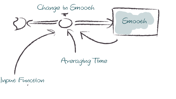
The SMOOTH function calculates the exponential average of the input, given the input function, an averaging time and, optionally, an initial value.
Signature: smooth(model, input_function, averaging_time, initial_value=None)
model: The model you are writing equations for
input_function: any model element
averaging_time: any model element
initial_value: a number, a model element or an expression. Left out, the average starts at the input
The SMOOTH operator is a shorthand for the following stock and flow structure and equations:
SMOOTH3 / SMOOTHN Functions
SMOOTH3 and SMOOTHN smooth the input in three or n stages, each with its share of the averaging time. The output reacts later than with SMOOTH and approaches the input in an S-curve rather than at once.
Signatures: smooth3(model, input_function, averaging_time, initial_value=None) and smoothn(model, input_function, averaging_time, order, initial_value=None)
averaging_time: any model element
initial_value: a number, a model element or an expression. Left out, the smooth starts at the input
order: a whole number between 1 and 255. smoothn keeps every stage at least one dt long, as in Stella
SQRT
Computes the Square root of an input expression.
Signature: sqrt(expression)
expression can be any element that returns a float value.
Simple Example:
STARTTIME Function
The STARTTIME function returns the models starttime.
Signature: starttime(model)
STEP Function
The STEP function generates a change of specified height, which occurs at a specified time: it is 0 before timestep and height from timestep on, as XMILE’s STEP is.
Signature: step(height, timestep)
height: any model element or a floating point number
timestep: any model element or a floating point number
STOPTIME Function
The STOPTIME function returns the models starttime.
Signature: stoptime(model)
TIME Function
The time function returns the current simulation time.
Signature: time()
TREND Function
The TREND function calculates the trend in the input, given the input, an averaging time and, optionally, the trend to start with. The TREND is defined to be the fractional change in input compared to the exponential average of input per averaging time. The TREND function thus estimates the growth rate of is input function.
Signature: trend(model, input_function, averaging_time, initial_trend=0.0)
model: The model you are writing equations for
input_function: any model element
averaging_time: any model element
initial_trend: the trend at the start, a number, a model element or an expression. The exponential average then starts at input / (1 + initial_trend * averaging_time), as in XMILE
The TREND operator is a shorthand for the following stock and flow structure and equations:
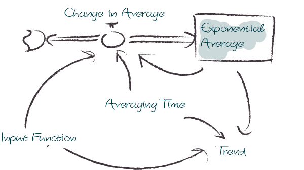
As an example, we set up a small model that has an input function that doubles every timestep - i.e the exponential growth rate is log 2 ≈ 0.69 and then apply the trend function to estimate the growth rate.
Here is a plot of the growth rate, which is constant:
This gives an input function which doubles in value on every timestep:
As expexted, the plot of the trend function converges to the input growth rate: